Determining Aquaculture Suitability

More information is available at this repository.

About

As the global population continues to grow exponentially, the sustainability of current protein sources can be called into question. Marine aquaculture provides a potential solution through this problem, as mapped by Gentry et al., where marine aquaculture potential was analyzed based on restraining factors such as bottom depth. They found that they could fulfill the global seafood demand by using less than 0.015% of the ocean area.

Set Up

Load libraries

library(terra) 
library(tidyverse)
library(tmap)
library(kableExtra) 
library(here)
library(sf)
library(stars)
library(viridis)
library(kableExtra)
library(here)

Read in data

# Bathymetry
bath <- rast(here('blogpost', 'aquaculture', 'data','depth.tif'))

# Exclusive Economic Zones
eez <- st_read(here('blogpost', 'aquaculture', 'data', 'wc_regions_clean.shp'))

Combine SST rasters into raster stack to read in data

# Sea surface temperature data
sst_2008 <- rast(here('blogpost', 'aquaculture','data','average_annual_sst_2008.tif'))
sst_2009 <- rast(here('blogpost', 'aquaculture','data','average_annual_sst_2009.tif'))
sst_2010 <- rast(here('blogpost', 'aquaculture','data','average_annual_sst_2010.tif'))
sst_2011 <- rast(here('blogpost', 'aquaculture','data','average_annual_sst_2011.tif'))
sst_2012 <- rast(here('blogpost', 'aquaculture','data','average_annual_sst_2012.tif'))

# Stack rasters using c()
sst_stack <- c(sst_2008, sst_2009, sst_2010, sst_2010, sst_2011, sst_2012)

Check CRS for suitable growing conditions

# Check CRS of sst_stack
st_crs(sst_stack) # no CRS

Coordinate Reference System:
  User input: WGS 84 
  wkt:
GEOGCRS["WGS 84",
    DATUM["unknown",
        ELLIPSOID["WGS84",6378137,298.257223563,
            LENGTHUNIT["metre",1,
                ID["EPSG",9001]]]],
    PRIMEM["Greenwich",0,
        ANGLEUNIT["degree",0.0174532925199433,
            ID["EPSG",9122]]],
    CS[ellipsoidal,2],
        AXIS["latitude",north,
            ORDER[1],
            ANGLEUNIT["degree",0.0174532925199433,
                ID["EPSG",9122]]],
        AXIS["longitude",east,
            ORDER[2],
            ANGLEUNIT["degree",0.0174532925199433,
                ID["EPSG",9122]]]]

# Match crs of sst to other CRS
sst_stack <- terra::project(sst_stack, "EPSG:4326")

# Check CRS between data sets
st_crs(bath) == st_crs(sst_stack)

[1] TRUE

st_crs(eez) == st_crs(sst_stack)

[1] TRUE

# Add warning to see if CRS match
if(st_crs(bath) == st_crs(eez) & st_crs(eez) == st_crs(sst_stack) & st_crs(bath) == st_crs(sst_stack)) {
  print("coordinate reference systems of datasets match")
}  else {
  warning("cooridnate reference systems to not match")
}

[1] "coordinate reference systems of datasets match"

Process Data

Find mean sea surface temperature

# Find mean SST from 2008-2012
sst_mean_k <- mean(sst_stack, na.rm = TRUE) # apply mean directly

# Convert from K to C by subtracting -273.15
sst_mean <- sst_mean_k - 273.15

Match depth and sea surface temperature

# Crop depth raster to match the extent of the SST raster
bath_crop <- crop(bath, ext(sst_mean)) # match extent

# Match resolutions of SST and depth
bath_rs <- resample(bath_crop, sst_mean, method = "near") # set method - week 4 lab

# Stack rasters for temperature and depth
stack_raster <- c(sst_mean, bath_rs)

# Check that the depth and SST match in:

# Resolution
resolution(sst_mean) == resolution(bath_rs)

[1] TRUE

# Extent
ext(sst_mean) == ext(bath_rs)

[1] TRUE

# CRS
st_crs(sst_mean) == st_crs(bath_rs)

[1] TRUE

# Visually check changes of cropped and resampled depth

# Cropped map
 tm_shape(bath_crop) +
  tm_raster(title = "Depth (m bsl)",
            palette = "Blues", midpoint = NA)  +
  tm_layout(main.title = "Crop Map",
            legend.outside = TRUE,
            legend.width = 5,
            title.size = 2)  +
  tm_compass(size = 2,
             position = c('left', 'top')) +
  tm_scale_bar(size = 2,
               position = c('right', 'bottom'))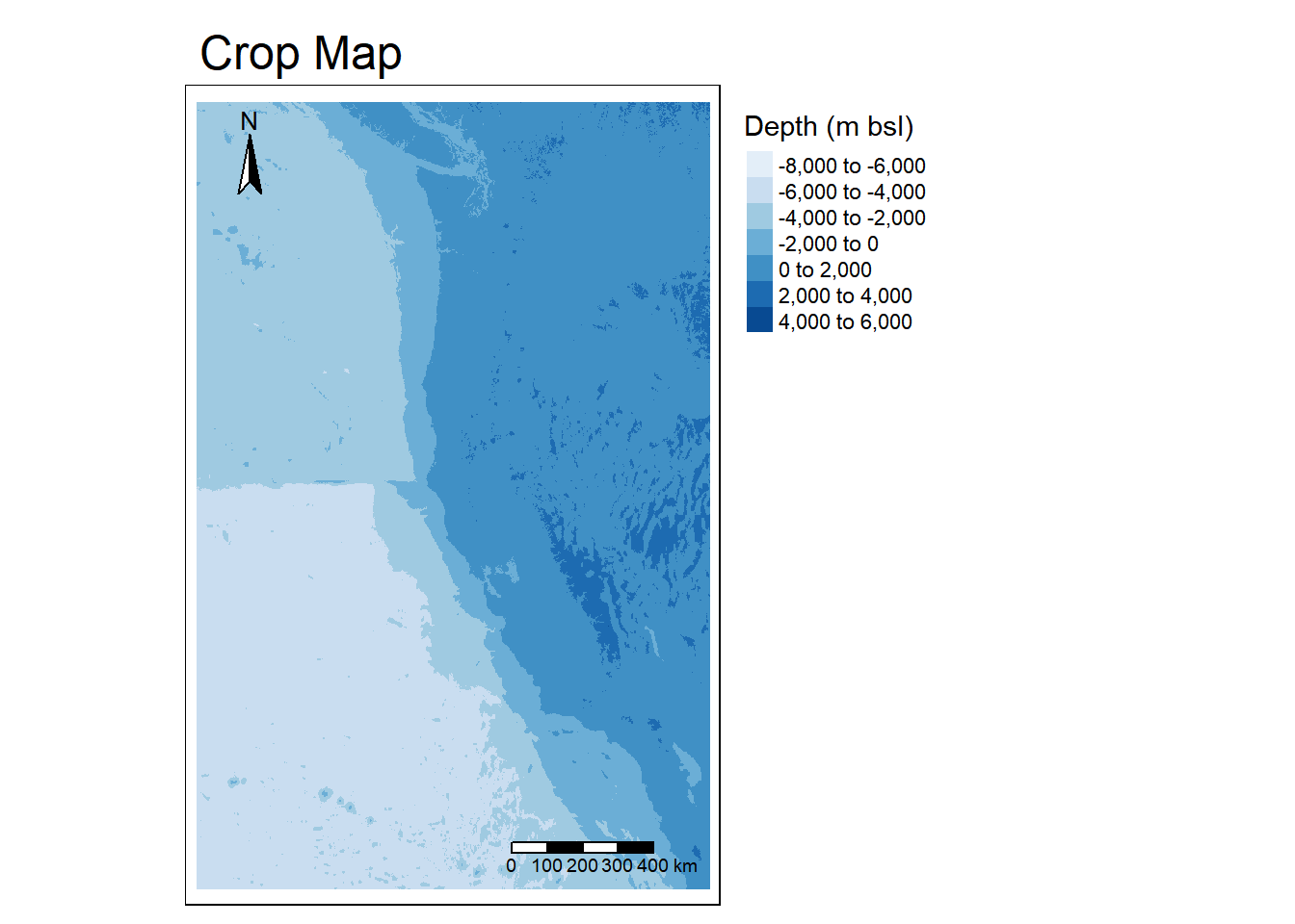

# Resampled map
 tm_shape(bath_rs) +
  tm_raster(title = "Depth (m bsl)",
            palette = "Blues", midpoint = NA)  +
  tm_layout(main.title = "Resampled Map",
            legend.outside = TRUE,
            legend.width = 5,
            title.size = 2) +
   tm_compass(size = 2,
             position = c('left', 'top')) +
   tm_scale_bar(size = 2,
               position = c('right', 'bottom'))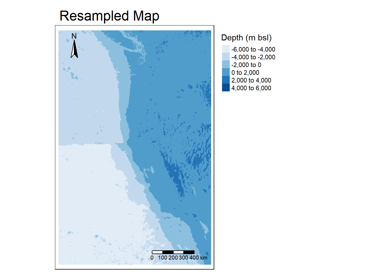

Find suitable locations

Recall Oyster optimal growing conditions:

• sea surface temperature: 11-30°C
• depth: 0-70 meters below sea level

Create reclassification matrices

# Reclassify sst and depth into oyster suitable locations

# Create reclassification matrix for sst
sst_reclass_mtx <- matrix(c(-Inf, 11, NA, # Temp below 11 degC is set to NA for unsuitable
                            11, 30, 1, # Temp from 11-30 degC is 1 indicating suitable
                            30, Inf, NA), # Temp above 30 degC is unsuitable, set to NA
                            ncol = 3, byrow = TRUE)

# Create reclassification matrix for depth
bath_reclass_mtx <- matrix(c(-Inf, -70, NA, # Depth below 70 mbsl set to NA indicating unsuitable
                             -70, 0, 1, # Depth from 0-70 mbsl is 1 for suitable
                             0, Inf, NA), # Depth greater than 0 m bsl set to NA for unsuitable
                             ncol = 3, byrow = TRUE)

Create inital plots of depth and temperature

# Use reclassification matrix to reclassify sst and depth

# Depth reclassification
bath_rcl <- classify(stack_raster$depth, rcl = bath_reclass_mtx) # select only depth

# Initial plot of depth
plot(bath_rcl)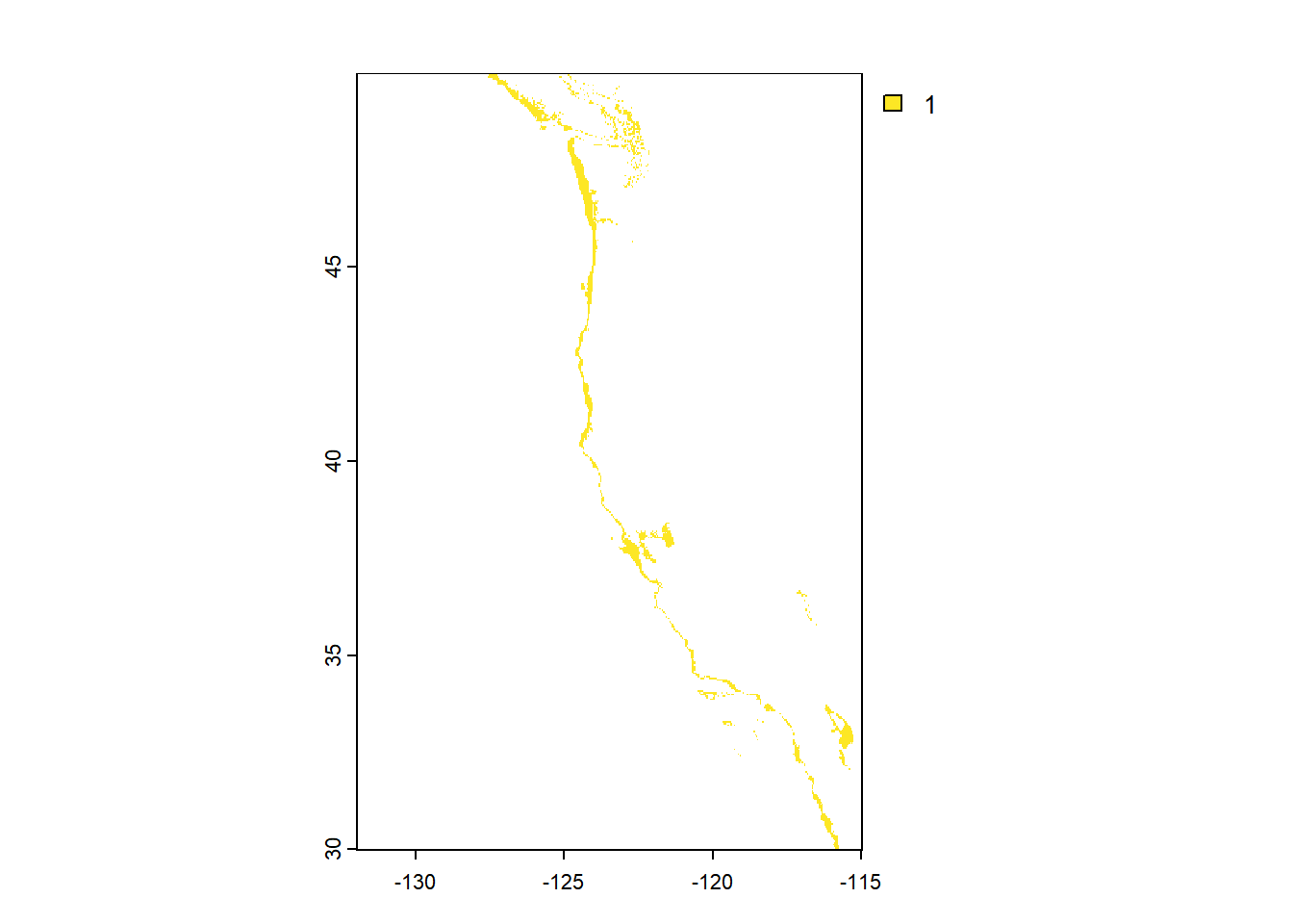

# SST/Temp reclassification
sst_rcl <- classify(stack_raster$mean, rcl = sst_reclass_mtx) # select only mean

# Initial plot of temperature
plot(sst_rcl)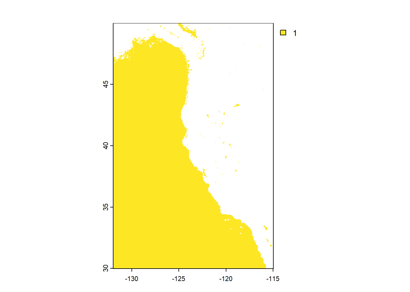

Inital plot of suitable oyster locations

# find locations that satisfy both SST and depth conditions

# Use lapp to multiply and determine conditions
# Anything multiplied by unsuitable will be 0, suitable will be 1

location <- lapp(c(bath_rcl, sst_rcl),
              fun = function(x,y){return(x*y)})

# Initial plot of suitable locations
plot(location)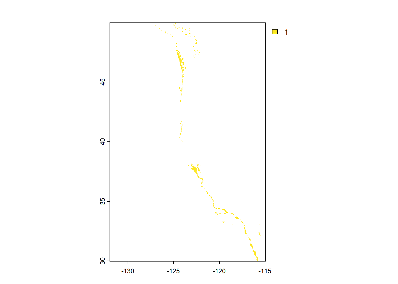

Determine the most suitable EEZ

• Find suitable cells and their area
• Find the total suitable area within each EEZ

# Select suitable cells within West Coast EEZs

# Mask location raster to EEZ locations
masked_location <- mask(location, eez)

# Initial plot
plot(masked_location)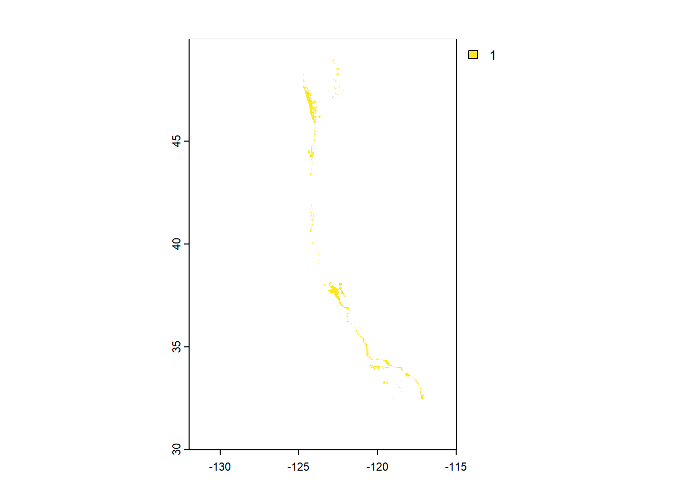

# Find the area of grid cells using cellSize

suitable_area <- cellSize(x = masked_location, # Selecting suitable locations from above
                 mask = TRUE, # When true, previous NA will carry over
                 unit = 'km') # Selecting km from data

# Initial plot
plot(suitable_area)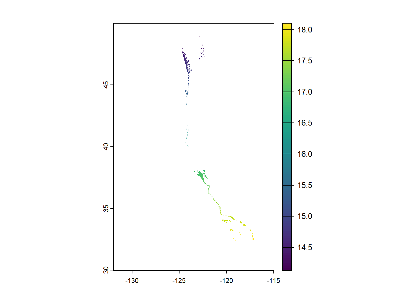

# Find the total suitable area within each EEZ

# Rasterize EEZ data
eez_raster <- rasterize(eez,
                        suitable_area, # to this raster
                        field = 'rgn') # Transfer values to each eez region

# Initial plot
plot(eez_raster)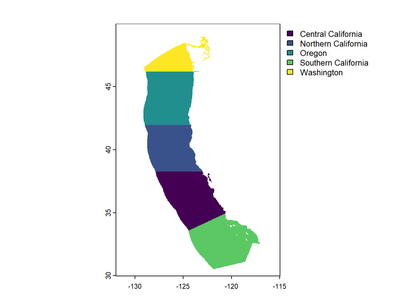

# Use zonal algebra to aggregate a grouping variable
eez_suitable <- zonal(x = suitable_area, 
                      z = eez_raster, # Raster representing zones
                      fun = 'sum', # To add up total area
                      na.rm = TRUE)


# Make table for suitable area by EEZ
kable(eez_suitable %>%
  st_drop_geometry() %>%
  select(Region = rgn,
         "Total Suitable Area(km<sup>2</sup>)" = area), caption = "Total suitable area of West Coast EEZs for oysters")

Total suitable area of West Coast EEZs for oysters

Region	Total Suitable Area(km2)
Central California	4973.782
Northern California	535.693
Oregon	1655.964
Southern California	3811.805
Washington	3750.691

Visualize suitable area for Oysters

# Map of suitable EEZ for oysters

tmap_mode("view")
# Suitable oyster area
oyster_map <- tm_shape(eez_raster) +
  tm_raster(title = "Total Suitable Area",
            palette= (c("#65AFFF", "#5899E2", "#335C81", "#4A85BF","#274060", "#1B2845"))) +
  
  # Add text labels and baselayer
  tm_shape(eez) +
  tm_text("rgn", size = 0.5) +
  tm_basemap("CartoDB.PositronNoLabels") +
  

# Map layout
  tm_layout(
            legend.outside = TRUE,
            main.title = "Suitable Area for Oysters\nby EEZ Region",
            title.size = 5,
            legend.width = 5,
            legend.outside.size = 0.5)

oyster_map

Generalize workflow by creating a function

# Function for any animal

suitable_animal_zone <- function(min_sst, max_sst, min_depth, max_depth, species_name) { # specify arguments
  
  # Reclassifying
  
    # Create reclassification matrix
  
      # Create reclassification matrix for sst
      sst_reclass_animal <- matrix(c(-Inf, min_sst, NA, 
                                min_sst, max_sst, 1, 
                                max_sst, Inf, NA), 
                                ncol = 3, byrow = TRUE)
    
      # Create reclassification matrix for depth
      bath_reclass_animal <- matrix(c(-Inf, min_depth, NA, 
                                 min_depth, max_depth, 1, 
                                 max_depth, Inf, NA), 
                                 ncol = 3, byrow = TRUE)
    # Apply reclassification
      
      # Stack rasters for temperature and depth
        stack_raster_animal <- c(sst_mean, bath_rs)
      
      # Depth reclassification
        bath_rcl_animal <- classify(stack_raster_animal$depth, rcl = bath_reclass_animal) 
      
      # SST/Temp reclassification
        sst_rcl_animal <- classify(stack_raster_animal$mean, rcl = sst_reclass_animal) 
  
  # Finding suitable area
  
      # Function to find suitable areas
      location_animal <- lapp(c(bath_rcl_animal, sst_rcl_animal),
                  fun = function(x,y){return(x*y)})
      
      # Mask location raster to EEZ locations
      masked_location_animal <- mask(location_animal, eez)
      
      # Find grid area
      suitable_area_animal <- cellSize(x = masked_location_animal, 
                     mask = TRUE, 
                     unit = 'km') 
      
      # Rasterize EEZ data
      eez_raster_animal <- rasterize(eez,
                            suitable_area_animal, 
                            field = 'rgn') 
  
  # Find suitable area by EEZ
  
  # Use zonal algebra to aggregate a grouping variable
      eez_suitable_animal <- zonal(x = suitable_area_animal, 
                          z = eez_raster_animal,
                          fun = 'sum',
                          na.rm = TRUE)

  # Print suitable area by EEZ
      kable(eez_suitable_animal %>%
  st_drop_geometry() %>%
  select(Region = rgn,
         "Total Suitable Area(km<sup>2</sup>)" = area), caption = "Total suitable area of West Coast EEZs")
      
  
 # Map of suitable EEZ for animal
tmap_mode("view")

# Suitable oyster area
tm_shape(eez_raster_animal) +
  tm_raster(title = "Total Suitable Area",
            palette= (c("#65AFFF", "#5899E2", "#335C81", "#4A85BF","#274060", "#1B2845"))) +
  
# Add text labels and baselayer
  tm_shape(eez) +
  tm_text("rgn", size = 0.5) +
  tm_basemap("CartoDB.PositronNoLabels") +

# Map layout
  tm_layout(
            legend.outside = TRUE,
            main.title = ("Suitable Area\nby EEZ Region"),
            title.size = 5,
            legend.width = 5,
            legend.outside.size = 0.5)
  
}

# Test function on oyster to confirm function 

suitable_animal_zone(min_sst = 11, max_sst = 30,
                   min_depth = -70, max_depth = 0, 
                   species_name = "Oyster")

Visualize suitable area for the American lobster

Now that we can reproduce our results with the function, apply it to our animal of choice:

Homarus americanus - American lobster - SST: 40-70F –> 4.4-21.1C - Depth: 4 - 50 m

# Plug in lobster values
suitable_animal_zone(min_sst = 4.4, max_sst = 21.1,
                   min_depth = 4, max_depth = 50, 
                   species_name = "American Lobster")

Citations

tribble(
  ~Data, ~Citation, ~Link,
  "Sea Life Base", "Palomares, M.L.D. and D. Pauly. Editors. 2024. SeaLifeBase. World Wide Web electronic publication. Retrieved: 11/14/24 from www.sealifebase.org, version (08/2024).","[Lobster Data ](https://www.sealifebase.ca/summary/Homarus-americanus.html)", 
   
  "Sea Surface Temperature Data", "NOAA Coral Reef Watch Version 3.1 (2018). Retrieved: 11/14/24", "[SST Data](https://coralreefwatch.noaa.gov/product/5km/index_5km_ssta.php)",
  
  "Bathymetry Data", "British Oceanographic Data Centere. Retrieved 11/14/24 from https://www.gebco.net/data_and_products/gridded_bathymetry_data/#area", "[Depth Data](https://www.gebco.net/data_and_products/gridded_bathymetry_data/#area)",
  
  "Cartographic Boundary Files - Shapefile Data", "United States Census Bureau. Retrieved 11/28/24 from https://www.census.gov/geographies/mapping-files/time-series/geo/carto-boundary-file.html", "[US Coast Data](https://www2.census.gov/geo/tiger/GENZ2018/shp/cb_2018_us_state_20m.zip)",
  
  "Exclusive Economic Zones Data", "MarineRegions.org. Retrieved 11/14/24 from https://www.marineregions.org/eez.php", "[EEZ Data](https://www.marineregions.org/downloads.php)",
  
  "American Lobster", "Defenders of Wildlife. Retrieved 11/28/24 from https://defenders-cci.org/landscape/climate-factsheets/ClimateChangeFS_American_Lobster.pdf", "[Lobster Temperature Range Data](defenders.org/climatechange)"
  
) %>%
  kable()

Data	Citation	Link
Sea Life Base	Palomares, M.L.D. and D. Pauly. Editors. 2024. SeaLifeBase. World Wide Web electronic publication. Retrieved: 11/14/24 from www.sealifebase.org, version (08/2024).	Lobster Data
Sea Surface Temperature Data	NOAA Coral Reef Watch Version 3.1 (2018). Retrieved: 11/14/24	SST Data
Bathymetry Data	British Oceanographic Data Centere. Retrieved 11/14/24 from https://www.gebco.net/data_and_products/gridded_bathymetry_data/#area	Depth Data
Cartographic Boundary Files - Shapefile Data	United States Census Bureau. Retrieved 11/28/24 from https://www.census.gov/geographies/mapping-files/time-series/geo/carto-boundary-file.html	US Coast Data
Exclusive Economic Zones Data	MarineRegions.org. Retrieved 11/14/24 from https://www.marineregions.org/eez.php	EEZ Data
American Lobster	Defenders of Wildlife. Retrieved 11/28/24 from https://defenders-cci.org/landscape/climate-factsheets/ClimateChangeFS_American_Lobster.pdf	Lobster Temperature Range Data

Note: Oyster data was provided on assignment website but can also be found at Sea Life Base.